9 replies to this topic

[raghava choudary]

Hi all,

 

I have concentration time profile after intramuscular (IM) administration and found that the absorption rate constant is much lower than the elimination rate constant ? Is is a flip-flop?

 

How to model the data with flip -flop kinetics ? I dont have the IV data for the compound !

 

Thanks in advance

 

Regards

 

RC

[serge guzy]

Hi all,

 

I have concentration time profile after intramuscular (IM) administration and found that the absorption rate constant is much lower than the elimination rate constant ? Is is a flip-flop?

 

How to model the data with flip -flop kinetics ? I dont have the IV data for the compound !

 

Thanks in advance

 

Regards

 

RC

Dear RC

You do modeling, not NCA. Therefore to me nothing different than usual. You fit the PK model to the data and you should get smaller Ka than Ke. I think the flip flop affects only the NCA output

. ke looks smaller than the corresponding one when giving IV because you still have absorption. On the other hand the upward part of the curve has information about ke too. That is why you callit  flip-flop.

When I used sustained released based data, I never had a problem to fit but only NCA results were completely wrong.

Serge

[smouksassi1]

Hi all,

 

I have concentration time profile after intramuscular (IM) administration and found that the absorption rate constant is much lower than the elimination rate constant ? Is is a flip-flop?

 

How to model the data with flip -flop kinetics ? I dont have the IV data for the compound !

 

Thanks in advance

 

Regards

 

RC

 

There is nothing special to do unless you want to force the model not to allow Ka to be < Ke or to force Ka to be always below Ke.

there is situation where Ka < Ke only on some subjects that is trickier and then the population estimates might not be pure Ka or pure Ke.

you need also to think about the half life and what does it mean and what is the reate limiting step. if Ka is the rate limiting step then what you see as terminal half life is more governed by the rate of relese from IM depot.

 

Samer

[raghava choudary]

Dear Serge / Samer,

 

Thank you for reply,

 

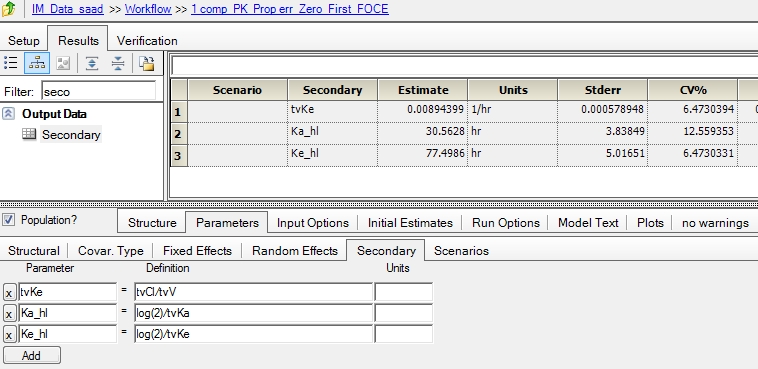
Modeled the IM data with one compartment parallel zero order and first order absorption with the following code that is mostly obtained from "Edit graphical" option.

 

The objective is to model the release of the drug from the IM site and also model the entry of drug in to the systemic circulation. the dose is 40 mg and so i have considered two dose points (both equal 40 mg) and parameter F is introduced. Please find the project attached for further details. The code is as follows:

test(){
                deriv(A1 = - (Cl * C) + (Aa * Ka))
                urinecpt(A0 = (Cl * C))
                deriv(Aa = - (Aa * Ka))
                C = A1 / V
                dosepoint(A1, bioavail = (F), duration = (tk0), idosevar = A1Dose, infdosevar = A1InfDose, infratevar = A1InfRate)
                dosepoint(Aa, bioavail = (1-F), idosevar = AaDose, infdosevar = AaInfDose, infratevar = AaInfRate)
                error(CEps = 0.342651)
                observe(CObs = C * (1 + CEps))
                stparm(V = tvV * exp(nV))
                stparm(Cl = tvCl * exp(nCl))
                stparm(Ka = tvKa * exp(nKa))
                stparm(F = tvF * exp(nF))
                stparm(tk0 = tvtk0 * exp(ntk0))
                fixef(tvV = c(, 8.37698, ))
                fixef(tvCl = c(, 0.073933, ))
                fixef(tvKa = c(, 0.0227794, ))
                fixef(tvF = c(, 0.686753, ))
                fixef(tvtk0 = c(, 303.547, ))
                ranef(diag(nV, nKa, nCl, nF, ntk0) = c(0.064958412, 0.54685374, 0.30482181, 0.078260499, 0.60039497))
}

The other question is, how to simulate the steady state data for this model ???

 

Thanks in advance 

 

Regards

 

RC

 

 IM_Data.phxproj   2.33MB   379 downloads

[raghava choudary]

Hi serge,

 

From the model code above, I have a F value of 0.68 , does it mean that 68 % of drug is following a zero order release in to the systemic circulation.

 

How do i calculate the half life of the drug ? do i have to use Ka for the calculation of apparent half life of the drug because the drug is following flip-flop kinetics ?

 

How to decide on the time to achieve steady state ? 

 

Thanks in advance.

 

Regards

 

RC

 

 

 

[Simon Davis]

Hi Raghav, dosing for 5-7 half lives is typically considered sufficient to reach steady state so I added the following to your model to get the the two half-lives calculated as secondary parameters.

 

With your data I think you could try 6 x thalf e.g. 6*30.5 = 186 h.  You can then run your simulation e.g. once daily dosing to 192 hours, and a copy to 360 hours (e.g 6*60h) and I think you will hit the same SS concs.  Let us know how you get on.

 

 Simon.

 

EDIT - I actually just tried it for you and I think that Ka’s half-life is 31 and Ke 77, so it’s slow but still not slower than Ke.  So I'd stick to using the Ke value and dose for at least 408 hours, preferably 552 hours, which gives C24 of 14730 and 14733 at 552h and 576h.

Attached Thumbnails

• 
• 

Edited by Simon Davis, 20 May 2016 - 11:33 AM.

[raghava choudary]

Hi Simon,

 

Thank you for the response,

 

attached project with simulations (dosing up to 552 hr) , predictive check, and bootstrap parameters. Since this is an intramuscular injection will it be useful if we select the dosing once a week based on the concentrations that are required?

 

Please guide if any major changes / modifications in the project. Thanks.

 

I have a different formulation of the same drug where the Ka half life is = 750 hr and Ke half life is 48 hrs. with the longer half life the drug would achieve steady state rapidly. when would be the next dose typically and in this the IM injection ?

 

Is there any option in phoenix to make shade areas for confidence intervals, any example files ?

 

Regards,

 

Raghav

 IM_T1_Data.phxproj   3.01MB   377 downloads

 

[raghava choudary]

Hi all,

 

I think can't use phoenix to simulate concentrations at steady state from the above model / project because phoenix is considering the elimination rate constant in the steady state concentrations. However, for this model Ka <<<< Ke (flip-flop) , i need to consider the apparent half life calculated from the absorption rate constant. Is there any way to simulate in phoenix the steady state concentrations ????

 

Regards,

 

RC

 

[Simon Davis]

Raghava, as demonstrated above you can see with multiple dosing the curve going up smoothsly to reach SS.

 

Such a simulation using your model paramters from fitting enables you to see empirically /confirm at what time we reach SS, (and the concentration profile predicted at that time).

 

Is there some other question that isn't clear or you need to ask?

  Simon.

[raghava choudary]

Raghava, as demonstrated above you can see with multiple dosing the curve going up smoothsly to reach SS.

 

Such a simulation using your model paramters from fitting enables you to see empirically /confirm at what time we reach SS, (and the concentration profile predicted at that time).

 

Is there some other question that isn't clear or you need to ask?

  Simon.

Hi Simon,

 

Greetings and Thank you for the response,

 

I am clear now about the simulation but i have a question on the model which was used. Can i use the split option for the dose on single compartment instead of using one dose point on Aa and one dose point on central compartment ???

 

The other question is do i have to use logit function on parameters like tvF (fraction that is released by zero order in the abobe model) ??

 

Thanks in advance,

 

Raghav