Jump to content


Photo
- - - - -

Lesson 4: Multiple Absorption Routes via Graphical Model Builder

PML Absorption graphical model

  • Please log in to reply
18 replies to this topic

#1 bwendt@certara.com

bwendt@certara.com

    Advanced Member

  • Administrators
  • 282 posts

Posted 21 November 2016 - 02:58 PM

On Nov 17th we have presented an exercise on multiple absorption routes where we used the graphical model builder in Phoenix to setup the model.

Here are the materials from this session.

Slide deck:

Attached File  PK43_multiple_absoprtion_routes.pdf   375.67KB   1717 downloads

Textual model:

Attached File  PK43_Multiple_Absorption_Routes.txt   1.23KB   1156 downloads

Link to recorded webinar:

https://certara.webe...6b6aba136d78e10


The responses to questions that were raised during the Q&A session are below:

Can you explain a little bit about all the plots that Phoenix spits out?
The Phoenix model object was designed to support both individual (WNL model) and Population PK/PD modeling (NLME mode), with standard output plots that have nomenclature similar to NONMEM (DV = dependent variable, IVAR = independent variable, TAD = Time After Dose, IPRED = individual predicted, PPRED = population predicted, and so on.) Similar names are used for the output plots when models are run in Individual mode. For a glossary description of the output plots for the Phoenix Model Object, see Help | Contents | Phoenix Model | Phoenix Model Run Modes, Engines, and Output | Phoenix Model Output | Plot output.

Will there still be a session for nonlinear kinetics?
Nonlinear kinetics has already been introduced in the following PML school sessions:
Lesson 1: Nonlinear Clearance
Lesson 2: Parent and Metabolite Kinetics
Nonlinear kinetics will also be covered extensively in future webinars in the series.

Can we model (i) discontinuous absorption in Phoenix how different is it from this model? (ii) Can we build transit compartments in the absorption phase?
Yes, discontinuous absorption can be modeled using “sequence” and “sleep” statements in a PML textual model. It is also possible to build transit compartments anywhere in a Phoenix text model. The syntax for these statements are described in Help | Documents | Phoenix Modeling Language Reference Guide.pdf.

How do you choose the error model?
Dan Weiner discussed this during the Q&A session of the webinar. Typically it is a good idea to start with the default Additive error model and work on model specification and initial error estimates. Once the structural model is finalized, the model can be fine-tuned by specifying the error model. The residual plots such as Ind IWRES vs IPRED, Ind IWRES vs IVAR, and QQIWRES can be used to identify patterns that might suggest a different error model is appropriate.

Why linear up and logdown calc method was used for NCA?
The linear up log down AUC calculation method uses the linear trapezoidal rule when concentrations are increasing, and the log method when concentrations are decreasing. Linear Up Log Down is a good choice when there are multiple peaks in the PK profile, as was the case here with both a fast absorption followed by a secondary delayed absorption.Many believe that the Linear Up Log Down method is the most accurate for interpolating between 2 adjacent datapoints because increase in concentration normally follow a linear path and decreases follow exponential decline. Thus the methodology for calculating AUC mirrors the expected profile path.

Where are the idosevar parameters set if you need to use them?
Idosevar gets created automatically by appending the word “Dose” to the name of the input column. For example, if your dosing input is “A1”, the corresponding idosevar is “A1Dose”. This is an internal variable name that can be used, in Secondary Parameter calculations. For example, if you wanted to calculate a dose-normalized Cmax using the above example, you could use the equation Cmax/A1Dose.

How to choose the initial value for Ka1 and Ka2?
One way to do this would be to calculate the slope of the log of the concentration values vs time. The slope of the first rise in log concentrations is an estimate of Ka1, and the slope of the second rise in log concentrations is an estimate of Ka2. These are crude estimates but generally good enough to achieve convergence. Another way is to use the Initial Estimates tab in the Phoenix model object. The second method was shown in the webinar. With all other parameters already having initial estimates via NCA methods, it was straightforward to find initial values for Ka1 and Ka2 using the overlay plot in the Initial Estimates tab.

Can unique initial estimates for multiple individuals be input using the graphics mode?
Yes. If you have multiple subjects in the input dataset and then use the Subject ID as a Sort variable in the model, you can go to Setup | Parameters, and then use an Internal Worksheet to specify initial parameter estimates for each Subject as shown below:
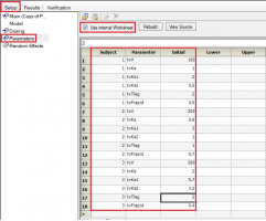
param_for_subject.png

Why use micro parameterization?
There is no particular reason why the micro parameterization was selected here. The PML language supports micro, macro and clearance parameterizations. Generally the clearance parameterization is preferred as it is numerically more stable.

Is it possible to have covariate effects on Ka for multiple dose sites?
Yes, it is possible to have covariate effects on any of the structural parameters in a Phoenix model – ka1 and ka2 in this case. For example, you might have sub-populations that are “fast absorbers” and “slow absorbers” ka2.

Is there a way to get the units to display for V or Ke like they do for Ka1, Ka2, and Tlag?
Dosing input units must be supplied to get units for V and Ke. The best way to do this is to create a Dosing input worksheet, with units in its column headers as shown below:

dose_units.png

Then, map this worksheet into the dosing panel under Setup | Dosing. You will then get output units for parameters that depend on the Dose, such as V and Ke:


dose_units2.png

When and How to select lower and upper in initial estimates?
Typically one starts with unbounded parameters, with only initial estimates. Boundaries may be applied in a secondary run of the model if the Thetas are unexpected. For example, a Lower boundary might be 0 or 0.0001 to ensure that the final parameter remains positive. An upper boundary might be set to ensure that a final estimate falls below an expected maximum value for a volume or rate constant.Bounds are not recommended when using Phoenix models, and are not allowed for algorithms such as QRPEM. If your model generates unexpected values for Thetas, you may consider re-parameterizing your model or determining if you have an error in the PML. The use of bounds forces limits on certain parameters, but can mask problems in your model code that should be remedied.

When during the model development process do you estimate the standard error and care whether you have a var-covar matrix estimated versus when to be guided by the return code.
For individual model fitting (WNL mode) one selects a residual error model that best achieves normaility of the residuals (based on the residual plots). This is part of the basic model development process, along with identifying the best structural model. A variance–covariance matrix is automatically generated based on the fitted model.
The standard error is only needed for the final model to estimate the variability in the parameter estimates. One recommendation is to turn off standard errors during model building and then only calculate standard errors only on the final model.
Return codes do not reflect problems with the selection of the residual error model per se. The ideal return code is 1. If it is over than 1, that suggests that the program is having some difficulty achieving convergence. The actual fit may be okay, or it the program may have converged to a local minimum. If you do have a return code other than 1, we suggest you rerun the model with different initial estimates and check to see if minus 2 times the log-likelihood (-2*LL) stays the same (the initial fit is likely okay) or is reduced (indicative of a local minimum with the prior fit).

Edited by bwendt@certara.com, 21 November 2016 - 03:15 PM.

  • Austingar, Donaldjet and Naitoeste like this

#2 Satish Sharan

Satish Sharan

    Newbie

  • Members
  • Pip
  • 3 posts

Posted 01 December 2016 - 04:39 PM

I thoroughly enjoyed excellent presentation by Bernd today morning and would greatly appreciate your thoughts on two questions related to this topic:

1) Can we change the rate of absorption in Oral compartment from 1st Order (Ka) to Zero order and be able to estimate the zero order absorption rate e.g. in cases of osmotic pumps?

2) How can we simultaneously fit one IV data and 5 Oral data with multiple dose levels?


Thanks!


#3 bwendt@certara.com

bwendt@certara.com

    Advanced Member

  • Administrators
  • 282 posts

Posted 01 December 2016 - 10:11 PM

Hi Satish,


thanks for your interest. Here are my responses:


re 1) you can change absorption options in the Graphical Model Builder. When you have the absorption compartment selected, you can see several options in the bottom panel, like zero-order-rate or zero-order duration:


zero_order.png


re 2) Please provide a dataset and we can show you how you can setup the model with different dose levels. It should be straightforward.


Cheers,


Bernd


#4 Satish Sharan

Satish Sharan

    Newbie

  • Members
  • Pip
  • 3 posts

Posted 05 December 2016 - 04:13 PM

Thanks Bernd!


#5 joybaker

joybaker

    Advanced Member

  • Val_Members
  • PipPipPip
  • 45 posts

Posted 01 December 2020 - 08:20 AM

Thank you for the recorded webinar that I can still learn it now. How my following question can still be answered.

Follow this question "Can unique initial estimates for multiple individuals be input using the graphics mode?", I have a data set consist of multiple formulation(same drug) and dose. And the parameters will be V,CL, Ka, tlag, K0. In the set up page the data will be sorted by "formulation" and "dose". Therefore each parameter has to be estimated by drug and dose.


How can I set V and CL parameter estimated from all formulation and dose (which make sense as for the same drug it will have similar distribution regardless of dose and formulation) and Ka,tlag and K0 estimated and sorted by formulation and dose (ie. one formulation set tlag=0 fixed while the other formulation as a parameter.)


PS. in the picture I used "drug" as sort tag, they are actually same drug but different formulation

Attached Thumbnails

  • 1.png


#6 bwendt@certara.com

bwendt@certara.com

    Advanced Member

  • Administrators
  • 282 posts

Posted 01 December 2020 - 10:04 AM

This setup reminds me of a one-stage IVIVC where you have a UIR from a reference formulation (e.g. IV or IR) with estimated V and Cl. Now you want to predict or fit the different absorption characteristics for a range of formulations. However, in your case you don't have a reference formulation, you just want typical values  for V and Cl instead, derived from all formulations. In population mode this is equivalent to not having random effects on V and Cl but on Ka, tlag and K0 (what is K0 stand for?). I am not sure this helps, but you may want to share your project file so that we could have a more detailed look.


Bernd


#7 joybaker

joybaker

    Advanced Member

  • Val_Members
  • PipPipPip
  • 45 posts

Posted 03 December 2020 - 04:03 AM

This setup reminds me of a one-stage IVIVC where you have a UIR from a reference formulation (e.g. IV or IR) with estimated V and Cl. Now you want to predict or fit the different absorption characteristics for a range of formulations. However, in your case you don't have a reference formulation, you just want typical values  for V and Cl instead, derived from all formulations. In population mode this is equivalent to not having random effects on V and Cl but on Ka, tlag and K0 (what is K0 stand for?). I am not sure this helps, but you may want to share your project file so that we could have a more detailed look.


Bernd


Thank you Bernd for you reply, I actually have a series of questions build on this multiple absorption example. This is a project I would like to replicate from the one who did it in NONMEN.


It is a three compartment model. Formulation A has first and zero order absorption in central compartment, first order with a "tlag", while formulation B has first order only. So the first question is how to set a variable tlag and duration for formulation A and tlag=0 and duration=0 (fixed) for formulation B?


The second question as I mentioned above, how to estimate V/CL/V2/V3/CL2/CL3 overall among various formulation and dose. And additionally fit Ka for each dose in formulation B, fit Ka/duration/tlag for all formulation A?

Output results would look like this:

                                              parameter#  estimates

CL                                                   1          xxx

V1                                                   2          xxx

CL2                                                 3          xxx

V2                                                   4          xxx

CL3                                                 5          xxx

V3                                                  6          xxx

tlag formulation B 10 mg               7       0 (fixed)

duration formulation B 10 mg        8       0 (fixed)

Ka formulation B 10 mg                9         xxx

tlag formulation B 25 mg               10       0 (fixed)

duration formulation B 25 mg        11       0 (fixed)

Ka formulation B 25 mg                12        xxx

tlag formulation B 40 mg               13       0 (fixed)

duration formulation B 40 mg        14       0 (fixed)

Ka formulation B 40 mg                15       xxx


tlag formulation A                         16       xxx

duration formulation A                 17       xxx

Ka formulation A                          18       xxx


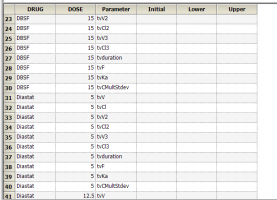
I have tried to exclude random effect for V/CL/V2/V3/CL2/CL3, however values were estimated so that they were the same for all ID in each formulation&dose but still different between formulation and dose (I don't know if you understand what I mean) . So V/CL/V2/V3/CL2/CL3 were estimated for all ID in each formulation&dose , while Ka/tlag/duration were estimated under each ID, which is still not as shown above. The tricky thing is in the main menu, when I sort data by  DOSE&DRUG&FOODSTATE, it will be sorted in all parameters.


Question three build upon the above, is it possible to add an between occasional variability (BOV) to each study (STUDYID)? 


It is followed with customised covariate setting, but I will leave it later before I can understand the basic model setting. Thank you.


#8 bwendt@certara.com

bwendt@certara.com

    Advanced Member

  • Administrators
  • 282 posts

Posted 03 December 2020 - 10:04 AM

Regarding the specifics on lag-time and zero-order duration you can use the dosepoint statement to deal with that, e.g.


dosepoint(Aa, tlag=Tlag, duration=Dur)

stparm(Tlag = tvTlag *TlagFlag*exp(nTlag))
stparm(Dur = tvDur *DurFlag*exp(nDur))
fcovariate(StudyID)
fcovariate(TlagFlag)
fcovariate(DurFlag)
fixef(tvTlag = c(,1,))
fixef(tvDur = c(,1,))
ranef(diag(nTlag, nDur) = c(1, 1))
 
You can add flags for Tlag and Dur as formulation specific covariates, e.g.  formulation-B==0, formulation-A=1. The flags can be incorporated as additional columns in your input set.


I am unable to comment on the behavior of the random effects, it would be good if you could share the project file to take a closer look. 


You can add occasional variability, e.g.:


stparm(Ka = tvKa * exp(nKa + nKax0*(StudyID==0) + nKax1*(StudyID==1)))


Hope, this helps.


Bernd


#9 joybaker

joybaker

    Advanced Member

  • Val_Members
  • PipPipPip
  • 45 posts

Posted 04 December 2020 - 07:10 AM

Regarding the specifics on lag-time and zero-order duration you can use the dosepoint statement to deal with that, e.g.


dosepoint(Aa, tlag=Tlag, duration=Dur)

stparm(Tlag = tvTlag *TlagFlag*exp(nTlag))
stparm(Dur = tvDur *DurFlag*exp(nDur))
fcovariate(StudyID)
fcovariate(TlagFlag)
fcovariate(DurFlag)
fixef(tvTlag = c(,1,))
fixef(tvDur = c(,1,))
ranef(diag(nTlag, nDur) = c(1, 1))
 
You can add flags for Tlag and Dur as formulation specific covariates, e.g.  formulation-B==0, formulation-A=1. The flags can be incorporated as additional columns in your input set.


I am unable to comment on the behavior of the random effects, it would be good if you could share the project file to take a closer look. 


You can add occasional variability, e.g.:


stparm(Ka = tvKa * exp(nKa + nKax0*(StudyID==0) + nKax1*(StudyID==1)))


Hope, this helps.


Bernd


Thank you Bernd. Didn't realise my attachment was not uploaded. I have also tried to add the durationFLAG and tlagFLAG in the model. I'm not sure if it works right. Even if tlag/durationFLAG are set to zero for formulation B, it seems still look for a value for tvtlag and tvduration. The output looks different from NONMEN as the example I typed in my previous log, where you can clearly see that tlag and duration are fixed to zero for formulation B.


Hope the file would explain more and look forward to your advice about the customised parameter group setting.

Attached Files


#10 bwendt@certara.com

bwendt@certara.com

    Advanced Member

  • Administrators
  • 282 posts

Posted 04 December 2020 - 09:47 AM

I think there were some issues with the data and a few missing covariates. Please see updated project file attached. Here are the steps that I took:


1. reintroduced tlagFLAG and durationFLAG

2 added a RESET column and used Input Options to switch it on

3. added DOSE,DRUG and FOODSTATE as categorical covariates

4. changed to a proportional residual error model


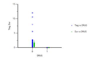
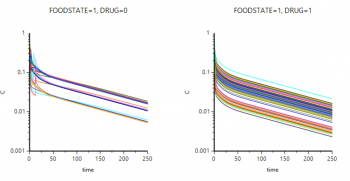
As you can see the flags do work:

DRUG.png

I would not say it is perfect, but it shoudl give you a good start.


FOODSTATE.png


Attached Files


#11 joybaker

joybaker

    Advanced Member

  • Val_Members
  • PipPipPip
  • 45 posts

Posted 29 December 2020 - 01:05 PM

I think there were some issues with the data and a few missing covariates. Please see updated project file attached. Here are the steps that I took:


1. reintroduced tlagFLAG and durationFLAG

2 added a RESET column and used Input Options to switch it on

3. added DOSE,DRUG and FOODSTATE as categorical covariates

4. changed to a proportional residual error model


As you can see the flags do work:

attachicon.gifDRUG.png

I would not say it is perfect, but it shoudl give you a good start.


attachicon.gifFOODSTATE.png


Thank you Bernd, I have made some progress in the model fitting, and I encounter new challenges. 


The 01 "3 compartment model" was used initially for the dataset. The fitting was ok, but I found the predicted Cmax was in general lower than the observed value. This is because several subjects showed double peaks and the model was fitting the first peak, and neglected the second peak, which was usually the real Cmax peak. This will affect my further simulation and prediction for alternative dosing regimen (evaluate Cmax and provide range), so I tried to focus on fitting the twin peaks (or catch the real Cmax) between 0-5 h.


So next I tried entrohepatic model and double absorption model, the latter similar as this topic. The fitting for 02 entrohepatic model is flatting the two peaks, which is not ideal (02 model has boundary for Cl, 03 model is the initial setting, give negative Cl and a trend for twin peaks). I am not sure if it is the problem of initial values or wrong model.


For the 04 double absorption model, I can see the two peak trend which is a good sign. But I can see the Cmax is still much underestimated. Also due to the variation (some subjects with only one peak, others have twin peaks), I feel the value of fixed parameters are wobbling as every time I ran the iteration, it will get a set of data slightly different. A few outliers in PopDV vs IPRED log also indicate problems.


Do you have any suggestion for improving this two models?

I understand the algorithm is try to find the best fit for overall data points. However I came across similar problems in PKPD model as well and I wonder what to do if I want to give best fit or more weight for certain critical data points during fitting? For example between 2-6 hours, or peak/valley of interests, which will be the key information for further prediction in large population or alternative doses.

Attached Thumbnails

  • 3 CMT Cmax under observed values.JPG

Attached Files


#12 bwendt@certara.com

bwendt@certara.com

    Advanced Member

  • Administrators
  • 282 posts

Posted 31 December 2020 - 01:13 PM

You can't overweigh a few or even a single data point when you fit a whole profile. In general, if you want to emphasize data points with high values, e.g. you want to fit Cmax well, you should go for uniform weighting, e.g. additive residual error, however, you will quickly find out through some diagnostic plots (e.g. CWRES vs IPRED) that you are missing out on data points with low values, hence a mixture of additive and multiplicative residual error model would be required. In your specific case, I received a hint from one of our developers and he pointed me to a power residual error model, which gave nice results, please see the attached project file and look at model 05.


Bernd


Attached File  fed_bw.phxproj   4.84MB   797 downloads


  • joybaker likes this

#13 joybaker

joybaker

    Advanced Member

  • Val_Members
  • PipPipPip
  • 45 posts

Posted 29 January 2021 - 11:25 AM

Thank you Bernd, I think this power model dose help improve for my purpose. I never think about using residual model other than additive, mutiplicative or mixture. Think should dig in more about the error model selection

You can't overweigh a few or even a single data point when you fit a whole profile. In general, if you want to emphasize data points with high values, e.g. you want to fit Cmax well, you should go for uniform weighting, e.g. additive residual error, however, you will quickly find out through some diagnostic plots (e.g. CWRES vs IPRED) that you are missing out on data points with low values, hence a mixture of additive and multiplicative residual error model would be required. In your specific case, I received a hint from one of our developers and he pointed me to a power residual error model, which gave nice results, please see the attached project file and look at model 05.


Bernd


attachicon.giffed_bw.phxproj


#14 joybaker

joybaker

    Advanced Member

  • Val_Members
  • PipPipPip
  • 45 posts

Posted 27 March 2021 - 04:37 AM

Dear Bernd,


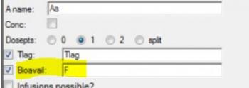
How can I add a bioavailability parameter on top of the two absorption route model, as the Frapid has been used in the bioabailability tab, but basically it is just a fraction of drug into Buccal and GI_tract. What if I want to see the bioavailablity of the fraction of drug in GI_tract in various dose/food state.


In the graphic mode, I was trying to use Frapid*Fbuccal and (1-ilogit(Frapid))*Fgitract for Buccal and GI_tract compartment, but it seems not working in that way. Do you know how I can do it?


Original code is written as the lesson:

# fractional dosing inputs
dosepoint(Buccal, bioavail = (Frapid), idosevar = BuccalDose)
dosepoint(GI_tract, tlag = (Tlag), bioavail = (1-Frapid), idosevar = GI_tractDose)

Attached Thumbnails

  • 1.JPG


#15 bwendt@certara.com

bwendt@certara.com

    Advanced Member

  • Administrators
  • 282 posts

Posted 29 March 2021 - 01:47 PM

Dear Joy,


I don't think you need an additional bioavailability term. If you are interested in different bioavailability between fasted and fed state, simply use the categorical covariate FOODSTATE and build a covariate relationship with F (or Frapid):


stparm(F = tvF * (1+dFdFOODSTATE1*(FOODSTATE==1)) * exp(nF))


Let me know if that helps.


Cheers,

Bernd


#16 joybaker

joybaker

    Advanced Member

  • Val_Members
  • PipPipPip
  • 45 posts

Posted 29 March 2021 - 02:39 PM

Dear Bernd,

Since I use f and 1-ilogit(f) for buccal and GItract, suppose I attach them to ADOSE/ADOSE1, that will make the overall bioavailability always equal to 1. However what I want to reflect is for example for 10 mg dose, there are only 8 mg (80%) goes to the system through Buccal and GItract. So how can I do that? Since the bioavailability tab is occupied by the fraction f.


Thank you for your help

jo


Dear Joy,


I don't think you need an additional bioavailability term. If you are interested in different bioavailability between fasted and fed state, simply use the categorical covariate FOODSTATE and build a covariate relationship with F (or Frapid):


stparm(F = tvF * (1+dFdFOODSTATE1*(FOODSTATE==1)) * exp(nF))


Let me know if that helps.


Cheers,

Bernd


#17 bwendt@certara.com

bwendt@certara.com

    Advanced Member

  • Administrators
  • 282 posts

Posted 31 March 2021 - 09:53 AM

Dear Joy,


You can have nested definitions of bioavailability. Please see another post in this forum:


https://support.cert...gic-lung-model/


Let me know if this more complex example helps you to resolve your issue. Otherwise, just post back here.


Cheers,


Bernd


#18 Ygsla

Ygsla

    Member

  • Members
  • PipPip
  • 11 posts

Posted 02 June 2022 - 12:54 PM

You can't overweigh a few or even a single data point when you fit a whole profile. In general, if you want to emphasize data points with high values, e.g. you want to fit Cmax well, you should go for uniform weighting, e.g. additive residual error, however, you will quickly find out through some diagnostic plots (e.g. CWRES vs IPRED) that you are missing out on data points with low values, hence a mixture of additive and multiplicative residual error model would be required. In your specific case, I received a hint from one of our developers and he pointed me to a power residual error model, which gave nice results, please see the attached project file and look at model 05.


Bernd


attachicon.giffed_bw.phxproj

Hi Bernd,


Attached file is not opening and showing error in Phoenix 8.3.1. Can u please attach again for reference?. I am facing problem in building PK model for my bimodular absorption profile.


Thanx!!

Ygsla


#19 bwendt@certara.com

bwendt@certara.com

    Advanced Member

  • Administrators
  • 282 posts

Posted 02 June 2022 - 03:13 PM

Attached File  fed_bw.phxproj   4.84MB   212 downloads


Hi Ygsla,


please find the project file attached.


Cheers,

Bernd


Also tagged with one or more of these keywords: PML, Absorption, graphical model

5 user(s) are reading this topic

0 members, 5 guests, 0 anonymous users